reading-notes
Matplotlib Tutorial
Introduction
matplotlib is probably the single most used Python package for 2D-graphics. It provides both a very quick way to visualize data from Python and publication-quality figures in many formats.
pyplot
pyplot provides a convenient interface to the matplotlib object-oriented plotting library. It is modeled closely after Matlab(TM). Therefore, the majority of plotting commands in pyplot have Matlab(TM) analogs with similar arguments. Important commands are explained with interactive examples.
Simple plot
n this section, we want to draw the cosine and sine functions on the same plot. Starting from the default settings
The first step is to get the data for the sine and cosine functions:
import numpy as np

X = np.linspace(-np.pi, np.pi, 256, endpoint=True)
C, S = np.cos(X), np.sin(X)
plt.plot(X,C)
plt.plot(X,S)

plt.show()
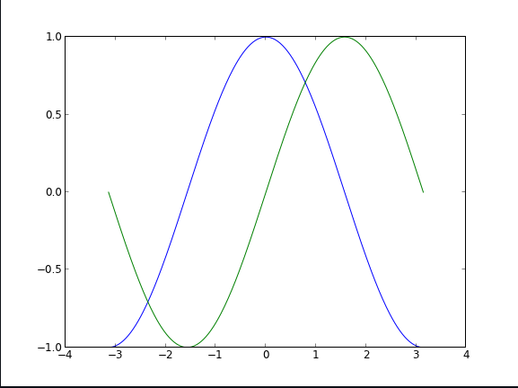
X is now a NumPy array with 256 values ranging from -π to +π (included). C is the cosine (256 values) and S is the sine (256 values).
Using defaults
Matplotlib comes with a set of default settings that allow customizing all kinds of properties. You can control the defaults of almost every property in matplotlib: figure size and dpi, line width, color and style, axes, axis and grid properties, text and font properties and so on. While matplotlib defaults are rather good in most cases, you may want to modify some properties for specific cases.
Changing colors and line widths
plt.figure(figsize=(10,6), dpi=80)
plt.plot(X, C, color="blue", linewidth=2.5, linestyle="-")
plt.plot(X, S, color="red",  linewidth=2.5, linestyle="-")
Setting limits
plt.xlim(X.min()*1.1, X.max()*1.1)
plt.ylim(C.min()*1.1, C.max()*1.1)
Annotate some points
Let’s annotate some interesting points using the annotate command. We choose the 2π/3 value and we want to annotate both the sine and the cosine. We’ll first draw a marker on the curve as well as a straight dotted line. Then, we’ll use the annotate command to display some text with an arrow.
t = 2*np.pi/3
plt.plot([t,t],[0,np.cos(t)], color ='blue', linewidth=1.5, linestyle="--")
plt.scatter([t,],[np.cos(t),], 50, color ='blue')

plt.annotate(r'$\sin(\frac{2\pi}{3})=\frac{\sqrt{3}}{2}$',
             xy=(t, np.sin(t)), xycoords='data',
             xytext=(+10, +30), textcoords='offset points', fontsize=16,
             arrowprops=dict(arrowstyle="->", connectionstyle="arc3,rad=.2"))

plt.plot([t,t],[0,np.sin(t)], color ='red', linewidth=1.5, linestyle="--")
plt.scatter([t,],[np.sin(t),], 50, color ='red')

plt.annotate(r'$\cos(\frac{2\pi}{3})=-\frac{1}{2}$',
             xy=(t, np.cos(t)), xycoords='data',
             xytext=(-90, -50), textcoords='offset points', fontsize=16,
             arrowprops=dict(arrowstyle="->", connectionstyle="arc3,rad=.2"))
Figures, Subplots and Axes
Figures
A figure is the windows in the GUI that has “Figure #” as title. Figures are numbered starting from 1 as opposed to the normal Python way starting from 0. This is clearly MATLAB-style. There are several parameters that determine what the figure looks like:
| Argument | Default | Description |
|---|---|---|
| num | 1 | number of figure |
| figsize | figure.figsize | figure size in in inches (width, height) |
| dpi | figure.dpi | resolution in dots per inch |
| facecolor | figure.facecolor | color of the drawing background |
| edgecolor | figure.edgecolor | color of edge around the drawing background |
| frameon | True | draw figure frame or not |